回归曲线图

查看 Markdown编辑此页

回归曲线图的简介

回归曲线图是一种在散点图基础上添加回归曲线的统计图表，用于展示两个或多个变量之间的数学关系和预测趋势。回归曲线通过数学算法拟合数据点，找出变量间的最佳函数关系，帮助分析数据的内在规律和进行趋势预测。

回归曲线图结合了散点图的数据分布展示能力和数学建模的预测功能，不仅能直观地显示数据点的分布，还能通过拟合曲线揭示变量间的潜在关系，是数据分析和科学研究中的重要工具。

常见的回归类型包括线性回归、多项式回归、指数回归、对数回归等，不同的回归方法适用于不同的数据模式和关系类型。

英文名：Regression Curve Chart

回归曲线图的构成

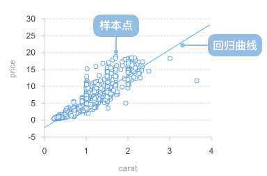
图表类型	回归曲线图
适合的数据	两个连续数据字段：一个自变量字段、一个因变量字段
功能	展示变量间的数学关系，识别数据趋势，进行预测分析
数据与图形的映射	自变量字段映射到横轴位置因变量字段映射到纵轴位置数据点显示原始观测值回归曲线显示拟合的数学关系
适合的数据条数	10-1000 条数据，数据点足够多才能有效进行回归分析

组成元素：

散点（Scatter Points）：表示原始数据观测值的点
回归曲线（Regression Curve）：通过数学算法拟合的趋势线
X 轴（X-axis）：水平坐标轴，通常表示自变量
Y 轴（Y-axis）：垂直坐标轴，通常表示因变量
回归方程（Regression Equation）：描述变量关系的数学公式
决定系数（R²）：衡量回归模型拟合优度的指标

回归曲线图的应用场景

适合的场景

例子 1: 线性关系数据分析

线性回归适用于展示两个变量之间的线性关系，如身高与体重、温度与销量等。

import { Chart } from '@antv/g2';
import { regressionLinear } from 'd3-regression';

const chart = new Chart({
  container: 'container',
  theme: 'classic',
});

chart.options({
  type: 'view',
  autoFit: true,
  data: {
    type: 'fetch',
    value: 'https://assets.antv.antgroup.com/g2/linear-regression.json',
  },
  children: [
    {
      type: 'point',
      encode: { x: (d) => d[0], y: (d) => d[1] },
      scale: { x: { domain: [0, 1] }, y: { domain: [0, 5] } },
      style: { fillOpacity: 0.75, fill: '#1890ff' },
    },
    {
      type: 'line',
      data: {
        transform: [
          {
            type: 'custom',
            callback: regressionLinear(),
          },
        ],
      },
      encode: { x: (d) => d[0], y: (d) => d[1] },
      style: { stroke: '#30BF78', lineWidth: 2 },
      labels: [
        {
          text: 'y = 1.7x + 3.01',
          selector: 'last',
          position: 'right',
          textAlign: 'end',
          dy: -8,
        },
      ],
      tooltip: false,
    },
  ],
  axis: {
    x: { title: '自变量 X' },
    y: { title: '因变量 Y' },
  },
});

chart.render();

说明：

散点显示原始数据分布
线性回归线揭示两变量间的线性关系
回归方程提供了精确的数学描述
适用于预测和趋势分析

例子 2: 非线性关系 - 二次回归

当数据呈现弯曲趋势时，可以使用二次回归（抛物线）来拟合数据。

import { Chart } from '@antv/g2';
import { regressionQuad } from 'd3-regression';

const chart = new Chart({
  container: 'container',
  theme: 'classic',
});

const data = [
  { x: -4, y: 5.2 },
  { x: -3, y: 2.8 },
  { x: -2, y: 1.5 },
  { x: -1, y: 0.8 },
  { x: 0, y: 0.5 },
  { x: 1, y: 0.8 },
  { x: 2, y: 1.5 },
  { x: 3, y: 2.8 },
  { x: 4, y: 5.2 },
];

chart.options({
  type: 'view',
  autoFit: true,
  data,
  children: [
    {
      type: 'point',
      encode: { x: 'x', y: 'y' },
      style: { fillOpacity: 0.75, fill: '#1890ff' },
    },
    {
      type: 'line',
      data: {
        transform: [
          {
            type: 'custom',
            callback: regressionQuad()
              .x((d) => d.x)
              .y((d) => d.y)
              .domain([-4, 4]),
          },
        ],
      },
      encode: { x: (d) => d[0], y: (d) => d[1] },
      style: { stroke: '#30BF78', lineWidth: 2 },
      labels: [
        {
          text: 'y = 0.3x² + 0.5',
          selector: 'last',
          textAlign: 'end',
          dy: -8,
        },
      ],
      tooltip: false,
    },
  ],
  axis: {
    x: { title: '自变量 X' },
    y: { title: '因变量 Y' },
  },
});

chart.render();

说明：

二次回归适合展示具有抛物线特征的数据关系
能够捕获数据的弯曲趋势和极值点
常用于物理学、经济学中的非线性关系分析

例子 3: 指数增长趋势分析

指数回归适用于展示指数增长或衰减的数据模式，如人口增长、细菌繁殖等。

import { Chart } from '@antv/g2';
import { regressionExp } from 'd3-regression';

const chart = new Chart({
  container: 'container',
  theme: 'classic',
});

chart.options({
  type: 'view',
  autoFit: true,
  data: {
    type: 'fetch',
    value: 'https://assets.antv.antgroup.com/g2/exponential-regression.json',
  },
  children: [
    {
      type: 'point',
      encode: { x: (d) => d[0], y: (d) => d[1] },
      scale: {
        x: { domain: [0, 18] },
        y: { domain: [0, 100000] },
      },
      style: { fillOpacity: 0.75, fill: '#1890ff' },
    },
    {
      type: 'line',
      data: {
        transform: [
          {
            type: 'custom',
            callback: regressionExp(),
          },
        ],
      },
      encode: {
        x: (d) => d[0],
        y: (d) => d[1],
        shape: 'smooth',
      },
      style: { stroke: '#30BF78', lineWidth: 2 },
      labels: [
        {
          text: 'y = 3477.32e^(0.18x)\nR² = 0.998',
          selector: 'last',
          textAlign: 'end',
          dy: -20,
        },
      ],
      tooltip: false,
    },
  ],
  axis: {
    x: { title: '时间' },
    y: {
      title: '数值',
      labelFormatter: '~s',
    },
  },
});

chart.render();

说明：

指数回归适合分析快速增长或衰减的趋势
R² 值接近 1 表示拟合效果很好
常用于预测具有指数特征的未来趋势

不适合的场景

例子 1: 数据点过少的情况

当数据点太少时，回归分析可能不够可靠，容易产生误导性的结论。

import { Chart } from '@antv/g2';
import { regressionLinear } from 'd3-regression';

const chart = new Chart({
  container: 'container',
  theme: 'classic',
});

const insufficientData = [
  { x: 1, y: 2 },
  { x: 3, y: 4 },
  { x: 5, y: 3 },
];

chart.options({
  type: 'view',
  autoFit: true,
  data: insufficientData,
  children: [
    {
      type: 'point',
      encode: { x: 'x', y: 'y' },
      style: {
        fillOpacity: 0.8,
        fill: '#ff4d4f',
        r: 8,
      },
    },
    {
      type: 'line',
      data: {
        transform: [
          {
            type: 'custom',
            callback: regressionLinear()
              .x((d) => d.x)
              .y((d) => d.y),
          },
        ],
      },
      encode: { x: (d) => d[0], y: (d) => d[1] },
      style: {
        stroke: '#ff4d4f',
        lineWidth: 2,
        strokeDasharray: [4, 4],
      },
      tooltip: false,
    },
  ],
  axis: {
    x: { title: '变量 X' },
    y: { title: '变量 Y' },
  },
  title: '不适合：数据点过少的回归分析',
});

chart.render();

问题说明：

仅有 3 个数据点，样本量不足
回归线的可靠性和预测能力有限
容易受到异常值的影响
建议至少需要 10 个以上的数据点进行回归分析

例子 2: 无明显相关关系的数据

当两个变量之间没有明显的相关关系时，强行添加回归线可能会误导分析。

import { Chart } from '@antv/g2';
import { regressionLinear } from 'd3-regression';

const chart = new Chart({
  container: 'container',
  theme: 'classic',
});

// 生成随机分布的数据（无相关关系）
const randomData = Array.from({ length: 30 }, (_, i) => ({
  x: Math.random() * 10,
  y: Math.random() * 10,
}));

chart.options({
  type: 'view',
  autoFit: true,
  data: randomData,
  children: [
    {
      type: 'point',
      encode: { x: 'x', y: 'y' },
      style: {
        fillOpacity: 0.8,
        fill: '#ff4d4f',
        r: 6,
      },
    },
    {
      type: 'line',
      data: {
        transform: [
          {
            type: 'custom',
            callback: regressionLinear()
              .x((d) => d.x)
              .y((d) => d.y),
          },
        ],
      },
      encode: { x: (d) => d[0], y: (d) => d[1] },
      style: {
        stroke: '#ff4d4f',
        lineWidth: 2,
        strokeDasharray: [4, 4],
      },
      labels: [
        {
          text: 'R² ≈ 0.02 (极低)',
          selector: 'last',
          textAlign: 'end',
          dy: -8,
        },
      ],
      tooltip: false,
    },
  ],
  axis: {
    x: { title: '变量 X' },
    y: { title: '变量 Y' },
  },
  title: '不适合：无相关关系的数据',
});

chart.render();

问题说明：

数据点呈现随机分布，无明显的趋势模式
R² 值极低，说明回归模型几乎无法解释变量关系
回归线没有实际意义，可能误导决策
应该先进行相关性分析，确认变量间存在关系后再进行回归

回归曲线图的扩展

多项式回归

当数据呈现复杂的弯曲趋势时，可以使用多项式回归来拟合更复杂的曲线。

import { Chart } from '@antv/g2';
import { regressionPoly } from 'd3-regression';

const chart = new Chart({
  container: 'container',
  theme: 'classic',
});

const polynomialData = [
  { x: 0, y: 140 },
  { x: 1, y: 149 },
  { x: 2, y: 159.6 },
  { x: 3, y: 159 },
  { x: 4, y: 155.9 },
  { x: 5, y: 169 },
  { x: 6, y: 162.9 },
  { x: 7, y: 169 },
  { x: 8, y: 180 },
];

chart.options({
  type: 'view',
  autoFit: true,
  data: polynomialData,
  children: [
    {
      type: 'point',
      encode: { x: 'x', y: 'y' },
      style: { fillOpacity: 0.75, fill: '#1890ff' },
    },
    {
      type: 'line',
      data: {
        transform: [
          {
            type: 'custom',
            callback: regressionPoly()
              .x((d) => d.x)
              .y((d) => d.y),
          },
        ],
      },
      encode: {
        x: (d) => d[0],
        y: (d) => d[1],
        shape: 'smooth',
      },
      style: { stroke: '#30BF78', lineWidth: 2 },
      labels: [
        {
          text: 'y = 0.24x³ - 3.00x² + 13.45x + 139.77\nR² = 0.92',
          selector: 'last',
          textAlign: 'end',
          dx: -8,
          dy: -20,
        },
      ],
      tooltip: false,
    },
  ],
  axis: {
    x: { title: '时间' },
    y: { title: '数值' },
  },
});

chart.render();

说明：

多项式回归能够拟合复杂的弯曲关系
适合处理具有多个波峰波谷的数据
需要注意避免过拟合问题

对数回归

对数回归适用于增长率逐渐减缓的数据模式。

import { Chart } from '@antv/g2';
import { regressionLog } from 'd3-regression';

const chart = new Chart({
  container: 'container',
  theme: 'classic',
});

chart.options({
  type: 'view',
  autoFit: true,
  data: {
    type: 'fetch',
    value: 'https://assets.antv.antgroup.com/g2/logarithmic-regression.json',
  },
  children: [
    {
      type: 'point',
      encode: { x: 'x', y: 'y' },
      scale: { x: { domain: [0, 35] } },
      style: { fillOpacity: 0.75, fill: '#1890ff' },
    },
    {
      type: 'line',
      data: {
        transform: [
          {
            type: 'custom',
            callback: regressionLog()
              .x((d) => d.x)
              .y((d) => d.y)
              .domain([0.81, 35]),
          },
        ],
      },
      encode: {
        x: (d) => d[0],
        y: (d) => d[1],
        shape: 'smooth',
      },
      style: { stroke: '#30BF78', lineWidth: 2 },
      labels: [
        {
          text: 'y = 0.881·ln(x) + 4.173\nR² = 0.958',
          selector: 'last',
          textAlign: 'end',
          dy: -20,
        },
      ],
      tooltip: false,
    },
  ],
  axis: {
    x: { title: '变量 X' },
    y: { title: '变量 Y' },
  },
});

chart.render();

说明：

对数回归适合展示边际递减效应
常用于分析学习曲线、收益递减等场景
能够处理增长率逐渐下降的数据模式

多变量回归对比

可以在同一图表中展示多种回归方法的对比效果。

import { Chart } from '@antv/g2';
import { regressionLinear, regressionQuad } from 'd3-regression';

const chart = new Chart({
  container: 'container',
  theme: 'classic',
});

const comparisonData = [
  { x: 1, y: 2.1 },
  { x: 2, y: 3.9 },
  { x: 3, y: 6.8 },
  { x: 4, y: 10.2 },
  { x: 5, y: 15.1 },
  { x: 6, y: 21.5 },
  { x: 7, y: 29.8 },
  { x: 8, y: 40.2 },
];

chart.options({
  type: 'view',
  autoFit: true,
  data: comparisonData,
  children: [
    {
      type: 'point',
      encode: { x: 'x', y: 'y' },
      style: {
        fillOpacity: 0.8,
        fill: '#1890ff',
        r: 6,
      },
    },
    // 线性回归
    {
      type: 'line',
      data: {
        transform: [
          {
            type: 'custom',
            callback: regressionLinear()
              .x((d) => d.x)
              .y((d) => d.y),
          },
        ],
      },
      encode: { x: (d) => d[0], y: (d) => d[1] },
      style: {
        stroke: '#ff4d4f',
        lineWidth: 2,
        strokeDasharray: [4, 4],
      },
      tooltip: false,
    },
    // 二次回归
    {
      type: 'line',
      data: {
        transform: [
          {
            type: 'custom',
            callback: regressionQuad()
              .x((d) => d.x)
              .y((d) => d.y),
          },
        ],
      },
      encode: { x: (d) => d[0], y: (d) => d[1] },
      style: {
        stroke: '#30BF78',
        lineWidth: 2,
      },
      tooltip: false,
    },
  ],
  axis: {
    x: { title: '变量 X' },
    y: { title: '变量 Y' },
  },
  legends: [
    {
      color: {
        position: 'top',
        itemMarker: (color, index) => {
          if (index === 0)
            return {
              symbol: 'line',
              style: { stroke: '#ff4d4f', strokeDasharray: [4, 4] },
            };
          if (index === 1)
            return { symbol: 'line', style: { stroke: '#30BF78' } };
        },
        data: [
          { color: '#ff4d4f', value: '线性回归' },
          { color: '#30BF78', value: '二次回归' },
        ],
      },
    },
  ],
});

chart.render();

说明：